Really, vertex welding is just a specialised form of collision detection. Each vertex needs to be checked against every other vertex to see if they're close together or not (and welded if they are). As such, a naive implementation runs in O(n^2) (or worse) time.
The first vertex welder I wrote was, well, slow. Welding a ~22,000 vertex mesh took over 12 seconds, and welding a smaller ~2300 vertex mesh took about 300ms. This was a completely unacceptable running time, as meshes are expected to run in the range of tens of thousands of vertices and a multi-minute loading time would be pure insanity.
That vertex welder was a very simple implementation: for each vertex, search every other vertex and weld if needed. If a weld occurred, then scan through the index buffer and make the necessary corrections. At worst, this algorithm ran in O(n^3) time, because it would need to loop through the index buffer each time a vertex was welded (and the index buffer's size for a freshly loaded COLLADA mesh is directly proportional to vertex count). At best, it was O(n^2).
I dumped that code and rewrote it from scratch, trading more memory usage for a better running time. I kept buffers which mapped vertices to welded vertices, and used this in a final, single loop over the index buffer to correct the indices. This brought the running time down to O((n^2+n)/2) (rather than between O(n^2) and O(n^3) like the old code). This dramatically improved running time: that 22,000 vertex mesh that took 12 seconds to load on the old code? 1.9 seconds on the new code.
Running the code through a profiler revealed a few performance hotspots. At the top of the list was an incredibly expensive square root that was being used in the distance calculations. Factoring out the square root and making some misc. performance changes increased the performance by a factor of 4.
But the algorithm was still too slow, O((n^2+n)/2) wasn't good enough. I needed to see if it would be possible to get it any faster. Rather than pine over micro optimisations in the code I had, I instead looked for a high-level algorithmic change.
The most common optimisation for dumb collision detection is spatial partitioning. Spatial partitioning involves splitting up the entities into groups based on their position. There are many constructs to achieve this, such as BSP trees and kd-trees.
I chose to use an octree. Octrees are a special case of kd-trees. Specifically, octrees are 3-dimensional kd-trees (and quadtrees are 2-dimensional kd-trees). Octrees are simple: divide up the search space into 8, equally sized, "octants". Each octant represents an eighth of the volume of the search space. Then for each octant, recursively split it into smaller and smaller octants until a desired limit is reached.
This diagram, courtesy of wikipedia, demonstrates nicely:
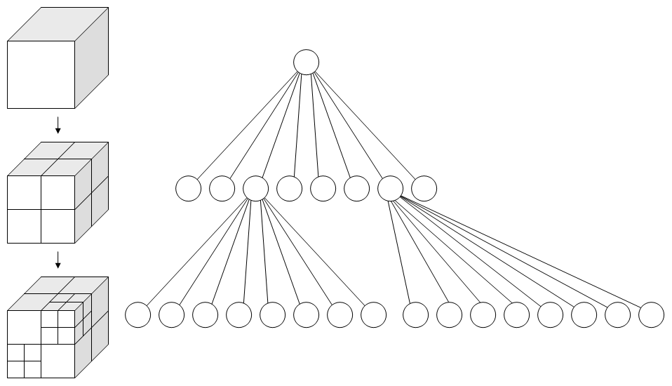
After the octree is constructed and all the vertices are divided into neat little groups based on spatial position, the welding can begin. Welding the mesh then simply consists of going through each octant in the octree, and welding the octant's vertices. Since the number of vertices in each octant is much smaller than the original, the welding is done much faster.
Usage of an octree reduces the time complexity from O(n^2) to average O(m(n / m)^2), where n is the total number of vertices and m is the total number of partitions in the octree. This can be simplified down to simply O(n^2/m). But what to choose for m? In other words, how many partitions should we create in the octree?
I chose a value of (sqrt(n) / 4). Why? No idea. It's a magic number, and it worked reasonably well. sqrt(n) would mean that the average number of vertices in each partition would be equal to the number of partitions. But the more partitions you create, the more overhead the octree has. But if you have too few partitions, the welding's going to take too long for each partition. It's a fine balance, and sqrt(n) / 4 seemed to work well.
This means that, when using the octree, the vertex welding algorithm is not quite O(n) linear time, but it's certainly a lot better than O(n^2). Here are the benchmark times:
~2,000 Vertex Ducky:
Original: 306ms
Profiled + Reoptimised + Octree: [Too fast to measure]
~12,000 Vertex Torus
Profiled + Reoptimised: 4181ms
Profiled + Reoptimised + Octree: 46ms
~22,000 Vertex Lunar Rover:
Original: 12768ms
Optimised: 1966ms
Profiled + Reoptimised: 468ms
Profiled + Reoptimised + Octree: 47ms
100,000 Vertex Sphere:
Profiled + Reoptimised: 489484ms
Profiled + Reoptimised + Octree: 686ms
As you can see, using the octree has resulted in a very significant improvement in speed. Completely welding a 100,000 vertex sphere now takes only 686ms compared to 489484ms, which is in excess of a 700x improvement in speed.


3 comments:
Very nice, thanks!
Hi my bro... just promo my blog about Welders
visit http://crazymig.com
thanks
Excellent post thank you kindly for sharing !
btw you can also use a hashmap and simply quantize point positions to the weld distance.
This takes ~N * (yourHashmapsTimeGrowthFactorHere), from experience its very close to N.
Post a Comment